In the previous tutorial (here) we concentrated on different ways to pass messages between cores which is one of the core mechanisms of parallelism. We saw that messages can be point to point, where only two cores are involved, or collective where every core is involved. The forms of communication that you select depends upon the problem you are trying to solve, and the example we considered (finding PI via the dartboard method) fitted very well with collective communications.
This tutorial will build upon tutorial two’s mechanisms of parallelism in order to take a higher level view of parallel codes by considering some of the common strategies (also known as patterns) that are available to parallel programmers and widely used. This tutorial will concentrate on geometric decomposition, which is also known as domain decomposition.
These tutorials use ePython, which is a subset of Python that runs on the Epiphany and allows us to quickly write and run some code. Before going any further if you have not yet used or installed ePython then it is worth following the instructions (here) which walks you though running a simple “hello world” ePython example on the Epiphany cores. If you installed ePython a while ago then it is worth ensuring that you are running the latest version, instructions for upgrading are available here.
Geometric decomposition
Splitting a problem up geometrically, and allocating different chunks of the data to different cores (or processes) is a very useful technique when there is one key data structure and the major organising principal of parallelism is splitting up of the data itself. In this strategy each core performs (roughly) the same instructions, just operating upon different data.

The diagram illustrates geometric decomposition in more detail, where an initially large 2D of data is split up into four chunks and each chunk is then distributed onto a different core. One of the key decisions for the parallel programmer is that of granularity, i.e. how many and how large these chunks should be. Granularity is very important because we want to maximise the amount of computation each core performs whilst minimising the communication between cores (which is an overhead of parallelism.) It is a trade-off, for instance in the diagram we only have four large chunks so only four cores can be utilised and these might have a very significant amount of computation to perform. At the other extreem, if we were to split the data into very many smaller chunks, then the cost of communication will likely dominate because each core only has a small amount of computation but very many cores results in lots of communications and cores are predominantly waiting for these communications to complete.
Jacobi iterative method
We are going to look at an algorithm very commonly used in HPC, namely an iterative method (the Jacobi method) to solve a partial differential equation (PDE.) We will be focussing on Laplace’s equation for diffusion, and you can think of a long pipe where we know the value of some pollutant at each end but not throughout the pipe iteself. Based upon this pipe and initial values we want to deduce how the pollution diffuses throughout. In order to solve this problem we split the pipe up into a number of distinct cells and set the values at the left most and right most cells (called the boundary conditions.) For every other cell, the value in that cell depends upon the values held in the neighbouring cells – which themselves depend upon their neighbours. The algorithm works in iterations, where each iteration will update all the unknown values and so progresses towards the final answer. At each iteration we calculate the residual which tells us how far away from the answer the current solution is and we will keep iterating until this residual is small enough to match a predetermined termination accuracy.
Halo swapping
In order to parallelise this problem we are going to split up the pipe geometrically and allocate different chunks to different Epiphany cores. I have already mentioned that the value at each cell depends upon its neighbouring cells, this is called the stencil and in this case we have a stencil size of one (we we only care about the direct neighbour in each direction.) What this tells us is that the majority of our computation will be local, but the calculation for the first and last points in a chunk (held by a core) will require a non-local neighbour’s value (held on a different core.)
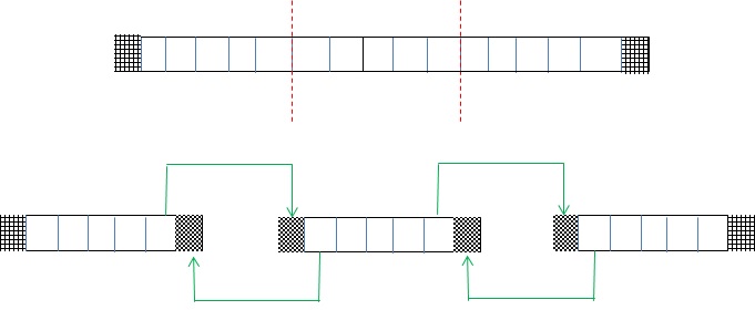
This is illustrated by the diagram, where the top image illustrates a pipe where we are solving 15 unknown pollution elements (empty boxes) and the left most and right most boundary condition (shaded) values are provided. This is then split up into three chunks in the lower illustration, each with 5 elements (empty boxes), and each chunk is allocated on a different core. It can be seen that for each chunk of data, there are actually seven elements – the five empty elements and one shaded on the left and one shaded on the right. These shaded elements are known as halos (or ghosts) and represent the neighbouring value required for the first and last local elements. A halo swap, where cores communicate neighbouring values, is performed en-mass at the start of each iteration and-so when it comes to the computation all the data a core requires is already present. Halo swapping results in fewer, larger messages (which is far more efficient than many smaller messages) and is a very common technique employed by HPC programmers.
ePython code
Now we have looked at some of the fundamental concepts underlying geometric decomposition and our example, it is time to get to the code!
import parallel

from math import sqrt


DATA_SIZE=100

MAX_ITS=100000


# Work out the amount of data to hold on this core

local_size=DATA_SIZE/numcores()

if local_size * numcores() != DATA_SIZE:

  if (coreid() < DATA_SIZE-local_size*numcores()): local_size=local_size+1


# Allocate the two arrays (two as this is Jacobi) we +2 to account for halos/boundary conditions

data=[0]*(local_size+2)

data_p1=[0]*(local_size+2)


# Set the initial conditions

i=0

while i<=local_size+1:

  data[i]=0.0

  i+=1


if coreid()==0: data[0]=1.0

if coreid()==numcores()-1: data[local_size+1]=10.0


# Compute the initial absolute residual

tmpnorm=0.0

i=1

while i<=local_size:

  tmpnorm=tmpnorm+(data[i]*2-data[i-1]-data[i+1])^2

  i+=1

tmpnorm=reduce(tmpnorm, "sum")

bnorm=sqrt(tmpnorm)


norm=1.0

its=0

while norm >= 1e-4 and its < MAX_ITS:

  # Halo swap to my left and right neighbours if I have them

  if (coreid() > 0): data[0]=sendrecv(data[1], coreid()-1)

  if (coreid() < numcores()-1): data[local_size+1]=sendrecv(data[local_size], coreid()+1)


  # Calculate current residual

  tmpnorm=0.0

  i=1

  while i<=local_size:

    tmpnorm=tmpnorm+(data[i]*2-data[i-1]-data[i+1])^2

    i+=1

  tmpnorm=reduce(tmpnorm, "sum")

  norm=sqrt(tmpnorm)/bnorm


  if coreid()==0 and its%1000 == 0: print "RNorm is "+norm+" at "+its+" iterations"


  # Performs the Jacobi iteration for Laplace

  i=1

  while i<=local_size:

    data_p1[i]=0.5* (data[i-1] + data[i+1])

    i+=1


  # Swap local data around for next iteration

  i=1

  while i<=local_size:

    data[i]=data_p1[i]
    i+=1

  its+=1


if coreid()==0: print "Completed in "+its+" iterations, RNorm="+norm
Copy this into a file named jacobi.py and execute epython jacobi.py (it is also provided in examples/jacobi.py), this will execute over all 16 Epiphany cores and you will see something like:
[device 0] RNorm is 1.000000 at 0 iterations

[device 0] RNorm is 0.004219 at 1000 iterations

[device 0] RNorm is 0.002365 at 2000 iterations

[device 0] RNorm is 0.001449 at 3000 iterations

[device 0] RNorm is 0.000893 at 4000 iterations

[device 0] RNorm is 0.000552 at 5000 iterations

[device 0] RNorm is 0.000341 at 6000 iterations

[device 0] RNorm is 0.000209 at 7000 iterations

[device 0] RNorm is 0.000129 at 8000 iterations

[device 0] Completed in 8500 iterations, RNorm=0.000100
At the top of the code the DATA_SIZE variable sets the global length of the pipe (100 in this case) and initially the cores will split up the pipe and determine how much data they hold locally (in local_size) before allocating the arrays data and data_p1 to hold their local data. You can see that each core actually allocates local_size+2 data elements, we have 2 extra elements for the left and right halos. The initial absolute residual is then calculated which deduces how far away from the final answer the initial setup lies, each core calculates the local residual and than the reduce collective communication call is used to sum these up to a global value.
Each core will then begin the Jacobi iteration itself and directly after this the halo swap is performed via the sendrecv communication calls which combine both sending to and receiving from a core into one operation. The residual (how far the solution is from the final answer) is calculated for each iteration (again using the reduce collective) and this is then taken relative to the initial residual to determine how far the solution has progressed which is one of our termination criteria.
This Jacobi method, whilst it is the slowest iterative solver, has some nice properties. One such property is that, given a fixed global problem size, irrespective of the number of cores you run with the progression towards the final answer at each iteration should be the same. You can display timing information via the -t command line argument, time a run with all 16 Epiphany cores and then run it only using 3 (-d 3 command line argument) cores, the runtime will increase because we have fewer cores doing more work.
No surprises so far, but remember at the start of the tutorial we discussed the granularity of the decomposition (fewer larger data chunks or many smaller chunks.) With this default pipe length of 100, 3 chunks is too few but actually 16 chunks is too many. Fixing the global problem size and varying the number of cores is an example of strong scaling, and running with abount 8 Epiphany cores is the optimum. Smaller core counts are slower because computations rule and larger core counts are slower because communication costs rule. Many people assume that simply throwing cores at a problem will speed it up, but as we have seen that is certainly not the case and often beyond a specific optimum (8 cores here), increasing the number of cores will actually slow down your code run.
If you double the global problem size (weak scaling) to 200 via the DATA_SIZE variable and rerun with 8 and 16 cores then you will see that 16 cores is faster than 8 cores in this scenario because there is still plenty of computational work for each core to perform at that granularity. In your home directory is a utility called ztemp.sh, which reports the heat of your Parallella, run this when the board is idle (for a baseline), then run the Jacobi example and, depending on how good your cooling solution is, you should see an increase in temperature when you run ztemp.sh again.
Summary
In this tutorial we have looked at geometric decomposition (also known as domain decomposition) which is a very common strategy for parallelism when your code is oriented around some key data structure(s) which can easily be split up. Iterative methods are very commonly used on supercomputers for solving systems of linear equations (such as Laplace’s PDE here) and Jacobi is one of these methods. Iterative methods, as well as many other computational algorithms, lend themselves towards geometric decomposition and this way of splitting the problem up feels very natural in these cases.
More information about Geometric decomposition can be found here and more information about iterative methods can be found here.
About the author
Dr Nick Brown works at EPCC, which is the UK’s leading centre for HPC. Nick currently develops weather models that run over many thousands of cores and has research interests in programming language and compiler design. More information here.